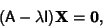
Let  be a linear transformation represented by a Matrix A. If there is a Vector
 such that
 |
(1) |
for some Scalar  , then is the eigenvalue of A with corresponding (right) Eigenvector
 . Letting A be a
  Matrix,
![\begin{displaymath}
\left[{\matrix{a_{11} & a_{12} & \cdots & a_{1k}\cr
a_{21} ...
...ots & \vdots\cr
a_{k1} & a_{k2} & \cdots & a_{kk}\cr}}\right]
\end{displaymath}](e_207.gif) |
(2) |
with eigenvalue , then the corresponding Eigenvectors satisfy
![\begin{displaymath}
\left[{\matrix{a_{11} & a_{12} & \cdots & a_{1k}\cr
a_{21} ...
...lambda \left[{\matrix{x_1\cr x_2\cr \vdots\cr x_k\cr}}\right],
\end{displaymath}](e_208.gif) |
(3) |
which is equivalent to the homogeneous system
![\begin{displaymath}
\left[{\matrix{a_{11}-\lambda & a_{12} & \cdots & a_{1k}\cr
...
...}}\right]
= \left[{\matrix{0\cr 0\cr \vdots\cr 0\cr}}\right].
\end{displaymath}](e_209.gif) |
(4) |
Equation (4) can be written compactly as
 |
(5) |
where I is the Identity Matrix.
As shown in Cramer's Rule, a system of linear equations has nontrivial solutions only if the Determinant
vanishes, so we obtain the Characteristic Equation
 |
(6) |
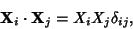
If all  s are different, then plugging these back in gives
  independent equations for the components
of each corresponding Eigenvector. The Eigenvectors will then be orthogonal and the system
is said to be nondegenerate. If the eigenvalues are
independent equations for the components
of each corresponding Eigenvector. The Eigenvectors will then be orthogonal and the system
is said to be nondegenerate. If the eigenvalues are  -fold Degenerate, then the system is said to be degenerate and
the Eigenvectors are not linearly independent. In such cases, the additional constraint that the
Eigenvectors be orthogonal,
-fold Degenerate, then the system is said to be degenerate and
the Eigenvectors are not linearly independent. In such cases, the additional constraint that the
Eigenvectors be orthogonal,
 |
(7) |
where  is the Kronecker Delta, can be applied to yield additional constraints, thus allowing solution
for the Eigenvectors.
is the Kronecker Delta, can be applied to yield additional constraints, thus allowing solution
for the Eigenvectors.
Assume A has nondegenerate eigenvalues
 and corresponding linearly independent
Eigenvectors
and corresponding linearly independent
Eigenvectors
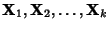 which can be denoted
![\begin{displaymath}
\left[{\matrix{x_{11}\cr x_{12}\cr \vdots\cr x_{1k}\cr}}\rig...
...eft[{\matrix{x_{k1}\cr x_{k2}\cr \vdots\cr x_{kk}\cr}}\right].
\end{displaymath}](e_217.gif) |
(8) |
Define the matrices composed of eigenvectors
![\begin{displaymath}
{\hbox{\sf P}} \equiv \left[{\matrix{{\bf X}_1 & {\bf X}_2 &...
...ots & \vdots\cr
x_{1k} & x_{2k} & \cdots & x_{kk}\cr}}\right]
\end{displaymath}](e_218.gif) |
(9) |
and eigenvalues
![\begin{displaymath}
{\hbox{\sf D}} \equiv \left[{\matrix{\lambda_1 & 0 & \cdots ...
...dots & \ddots & \vdots\cr 0 & 0 & \cdots & \lambda_k}}\right],
\end{displaymath}](e_219.gif) |
(10) |
where
 is a Diagonal Matrix. Then
so
 |
(12) |
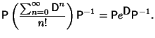
Furthermore,
By induction, it follows that for  ,
,
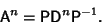 |
(14) |
The inverse of A is
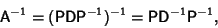 |
(15) |
where the inverse of the Diagonal Matrix D is trivially given by
![\begin{displaymath}
{\hbox{\sf D}}^{-1}= {1\over k}
\left[{\matrix{{\lambda_1}^...
...\ddots & \vdots\cr 0 & 0 & \cdots & {\lambda_k}^{-1}}}\right].
\end{displaymath}](e_235.gif) |
(16) |
Equation (14) therefore holds for both Positive and Negative .
A further remarkable result involving the matrices
 and
follows from the definition
and
follows from the definition
Since D is a Diagonal Matrix,
 can be found using
![\begin{displaymath}
{\hbox{\sf D}}^n = \left[{\matrix{{\lambda_1}^n & 0 & \cdots...
...\ddots & \vdots\cr 0 & 0 & \cdots & {\lambda_k}^n\cr}}\right].
\end{displaymath}](e_246.gif) |
(19) |
Assume we know the eigenvalue for
 |
(20) |
Adding a constant times the Identity Matrix to A,
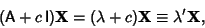 |
(21) |
so the new eigenvalues equal the old plus  . Multiplying A by a constant
 |
(22) |
so the new eigenvalues are the old multiplied by .
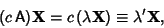
Now consider a Similarity Transformation of A. Let
 be the Determinant of A, then
so the eigenvalues are the same as for A.
See also Brauer's Theorem,
Condition Number, Eigenfunction, Eigenvector, Frobenius Theorem,
Gersgorin Circle Theorem, Lyapunov's First Theorem, Lyapunov's Second Theorem,
Ostrowski's Theorem, Perron's Theorem, Perron-Frobenius Theorem, Poincaré Separation
Theorem, Random Matrix,
Schur's Inequalities, Sturmian Separation Theorem, Sylvester's
Inertia Law, Wielandt's Theorem
References
Arfken, G. ``Eigenvectors, Eigenvalues.'' §4.7 in Mathematical Methods for Physicists, 3rd ed.
Orlando, FL: Academic Press, pp. 229-237, 1985.
Nash, J. C. ``The Algebraic Eigenvalue Problem.''
Ch. 9 in Compact Numerical Methods for Computers: Linear Algebra
and Function Minimisation, 2nd ed. Bristol, England: Adam Hilger, pp. 102-118, 1990.
Press, W. H.; Flannery, B. P.; Teukolsky, S. A.; and Vetterling, W. T. ``Eigensystems.'' Ch. 11 in
Numerical Recipes in FORTRAN: The Art of Scientific Computing, 2nd ed. Cambridge, England:
Cambridge University Press, pp. 449-489, 1992.
© 1996-9 Eric W. Weisstein
1999-05-25
![$\displaystyle \left[\begin{array}{cccc}\lambda_1x_{11} & \lambda_2x_{21} & \cdo...
... \lambda_1x_{1k} & \lambda_2x_{2k} & \cdots & \lambda_kx_{kk}\end{array}\right]$](e_225.gif)
![$\displaystyle \left[\begin{array}{cccc}x_{11} & x_{21} & \cdots & x_{k1}\\ x_{...
...dots & \vdots & \ddots & \vdots\\ 0 & 0 & \cdots & \lambda_k\end{array}\right]$](e_226.gif)
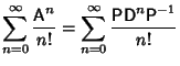
![$\displaystyle \sum_{n=0}^\infty {{\hbox{\sf D}}^n\over n!} = \sum_{n=0}^\infty ...
... & \vdots & \ddots & \vdots\\ 0 & 0 & \cdots & {\lambda_k}^n\end{array}\right]$](e_242.gif)
![$\displaystyle \left[\begin{array}{cccc}\sum_{n=0}^\infty {{\lambda_1}^n\over n!...
...\ 0 & 0 & \cdots & \sum_{n=0}^\infty {{\lambda_k}^n\over n!}\end{array}\right]$](e_243.gif)
![$\displaystyle \left[\begin{array}{cccc}e^{\lambda_1} & 0 & \cdots & 0\\ 0 & e^...
...& \vdots & \ddots & \vdots\\ 0 & 0 & \cdots & e^{\lambda_k}\end{array}\right],$](e_244.gif)