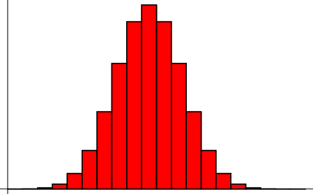
The probability of  successes in
  Bernoulli Trials is
 |
(1) |
The probability of obtaining more successes than the  observed is
 |
(2) |
where
 |
(3) |
 is the Beta Function, and
  is the incomplete Beta Function. The Characteristic
Function is
 |
(4) |
The Moment-Generating Function  for the distribution is
The Mean is
 |
(8) |
The Moments about 0 are
so the Moments about the Mean are
The Skewness and Kurtosis are
An approximation to the Bernoulli distribution for large  can be obtained by expanding about the value
  where
where
 is a maximum, i.e., where
  . Since the Logarithm function is Monotonic, we can instead choose to expand the Logarithm. Let
 , then
![\begin{displaymath}
\ln[P(n)] = \ln [P(\tilde n)]+B_1\eta +{\textstyle{1\over 2}}B_2\eta^2+{\textstyle{1\over 3!}} B_3\eta^3+\ldots,
\end{displaymath}](b_1376.gif) |
(18) |
where
![\begin{displaymath}
B_k\equiv \left[{d^k \ln[P(n)]\over dn^k}\right]_{n=\tilde n}.
\end{displaymath}](b_1377.gif) |
(19) |
But we are expanding about the maximum, so, by definition,
![\begin{displaymath}
B_1 =\left[{d \ln[P(n)]\over dn}\right]_{n=\tilde n} = 0.
\end{displaymath}](b_1378.gif) |
(20) |
This also means that  is negative, so we can write
  . Now, taking the Logarithm of (1) gives
![\begin{displaymath}
\ln[P(n)] = \ln N!-\ln n!-\ln(N-n)!+n\ln p+(N-n)\ln q.
\end{displaymath}](b_1380.gif) |
(21) |
For large  and
and  we can use Stirling's Approximation
 |
(22) |
so
and
![\begin{displaymath}
{d\ln[P(n)]\over dn} \approx -\ln n+\ln(N-n)+\ln p-\ln q.
\end{displaymath}](b_1389.gif) |
(25) |
To find  , set this expression to 0 and solve for
  ,
,
 |
(26) |
 |
(27) |
 |
(28) |
 |
(29) |
since  . We can now find the terms in the expansion
Now, treating the distribution as continuous,
 |
(33) |
Since each term is of order
 smaller than the previous, we can ignore terms higher than
  , so
, so
 |
(34) |
The probability must be normalized, so
 |
(35) |
and
Defining
 ,
,
![\begin{displaymath}
P(n) = {1\over\sigma\sqrt{2\pi}}\mathop{\rm exp}\nolimits \left[{-{(n-\tilde n)^2\over 2\sigma^2}}\right],
\end{displaymath}](b_1414.gif) |
(37) |
which is a Gaussian Distribution. For  , a different approximation procedure shows that the binomial
distribution approaches the Poisson Distribution. The first Cumulant is
 |
(38) |
and subsequent Cumulants are given by the Recurrence Relation
 |
(39) |
Let  and
and  be independent binomial Random Variables characterized by parameters
  and
and  . The
Conditional Probability of
  given that
  is
is

|
|

|
(40) |
Note that this is a Hypergeometric Distribution!
See also de Moivre-Laplace Theorem, Hypergeometric Distribution, Negative Binomial Distribution
References
Beyer, W. H. CRC Standard Mathematical Tables, 28th ed. Boca Raton, FL: CRC Press, p. 531, 1987.
Press, W. H.; Flannery, B. P.; Teukolsky, S. A.; and Vetterling, W. T.
``Incomplete Beta Function, Student's Distribution, F-Distribution, Cumulative Binomial Distribution.'' §6.2 in
Numerical Recipes in FORTRAN: The Art of Scientific Computing, 2nd ed. Cambridge, England:
Cambridge University Press, pp. 219-223, 1992.
Spiegel, M. R. Theory and Problems of Probability and Statistics. New York: McGraw-Hill, p. 108-109, 1992.
© 1996-9 Eric W. Weisstein
1999-05-26

![]() successes in
successes in ![]() Bernoulli Trials is
Bernoulli Trials is


![$\displaystyle {\mu_3\over\sigma^3} = {Np(1-p)(1-2p)\over [Np(1-p)]^{3/2}}$](b_1369.gif)

![$\displaystyle {d[\ln(n!)]\over dn}$](b_1383.gif)
![$\displaystyle {d[\ln(N-n)!]\over dn}$](b_1385.gif)
![$\displaystyle {d\over dn} [(N-n)\ln(N-n)-(N-n)]$](b_1386.gif)
![$\displaystyle \left[{-\ln(N-n)+(N-n) {-1\over N-n} +1}\right]$](b_1387.gif)
![$\displaystyle \left[{d^2 \ln[P(n)]\over dn^2}\right]_{n=\tilde n}
= -{1\over \tilde n}-{1\over N-\tilde n}$](b_1395.gif)


![$\displaystyle \left[{d^3 \ln[P(n)]\over dn^3}\right]_{n=\tilde n}
= {1\over \tilde n^2}-{1\over(N-\tilde n)^2}$](b_1399.gif)


![$\displaystyle \left[{d^4 \ln[P(n)]\over dn^4}\right]_{n=\tilde n}
= -{2\over \tilde n^3}-{2\over(n-\tilde n)^3}$](b_1402.gif)


![$\displaystyle {2[p^2-p(1-p)+(1-2p+p^2)]\over N^3p^3(1-p^3)}$](b_1405.gif)


![$\displaystyle {1\over \sqrt{2\pi Npq}}\mathop{\rm exp}\nolimits \left[{-{(n-Np)^2\over 2Npq}}\right].$](b_1412.gif)
![]() and
and ![]() be independent binomial Random Variables characterized by parameters
be independent binomial Random Variables characterized by parameters ![]() and
and ![]() . The
Conditional Probability of
. The
Conditional Probability of ![]() given that
given that ![]() is
is