|
|
|
The logistic equation (sometimes called the Verhulst Model since it was first published in 1845 by the Belgian
P.-F. Verhulst) is defined by
| (1) |
| (2) |
| (3) |
| (4) |
| (5) |
| (6) |
| (7) |
| (8) |
| (9) |
| (10) |
| (11) |
|
|
|
|
|
|
|
|
|
|
|
|
|
|
|
|
|
|
|
|
|
|
|
|
|
|
|
|
|
(12) |
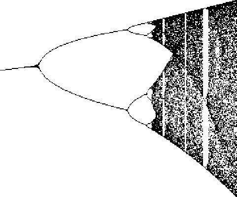
A table of the Cycle type and value of ![]() at which the cycle
at which the cycle ![]() appears is given below.
appears is given below.
| cycle ( |
||
| 1 | 2 | 3 |
| 2 | 4 | 3.449490 |
| 3 | 8 | 3.544090 |
| 4 | 16 | 3.564407 |
| 5 | 32 | 3.568750 |
| 6 | 64 | 3.56969 |
| 7 | 128 | 3.56989 |
| 8 | 256 | 3.569934 |
| 9 | 512 | 3.569943 |
| 10 | 1024 | 3.5699451 |
| 11 | 2048 | 3.569945557 |
| acc. pt. | 3.569945672 |
For additional values, see Rasband (1990, p. 23). Note that the table in Tabor (1989, p. 222) is incorrect, as is the
![]() entry in Lauwerier (1991). In the middle of the complexity, a window suddenly appears with a regular period like 3
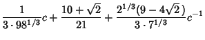
or 7 as a result of Mode Locking. The period 3 Bifurcation occurs at
entry in Lauwerier (1991). In the middle of the complexity, a window suddenly appears with a regular period like 3
or 7 as a result of Mode Locking. The period 3 Bifurcation occurs at
![]() , as is
derived below. Following the 3-Cycle, the Period Doublings then begin
again with Cycles of 6, 12, ...and 7, 14, 28, ..., and then once again break off to
Chaos.
, as is
derived below. Following the 3-Cycle, the Period Doublings then begin
again with Cycles of 6, 12, ...and 7, 14, 28, ..., and then once again break off to
Chaos.
A set of ![]() equations which can be solved to give the onset of an arbitrary
equations which can be solved to give the onset of an arbitrary ![]() -cycle (Saha and Strogatz
1995) is
-cycle (Saha and Strogatz
1995) is
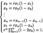 |
(13) |
For ![]() , the solutions (
, the solutions (![]() , ...,
, ..., ![]() ,
, ![]() ) are (0, 0,
) are (0, 0, ![]() ) and (
) and (![]() ,
, ![]() , 3), so the desired
Bifurcation occurs at
, 3), so the desired
Bifurcation occurs at ![]() . Taking
. Taking ![]() gives
gives
![$\displaystyle {d[f^3(x)]\over dx}$](l2_777.gif) |
![$\displaystyle {d[f^3(x)]\over d[f^2(x)]} {d[f^2(x)]\over d[f(x)]} {d[f(x)]\over dx}$](l2_778.gif) |
||
![$\displaystyle {d[f(z)]\over dz} {d[f(y)]\over dy} {d[f(x)]\over dx}$](l2_779.gif) |
|||
| (14) |
 |
|||
 |
|||
 |
(15) | ||
 |
|||
 |
|||
 |
(16) | ||
 |
(17) | ||
| (18) |
| (19) |
| (20) | |||
| (21) | |||
| (22) | |||
| (23) |
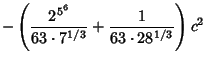
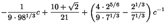
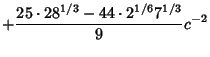
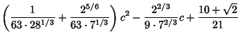
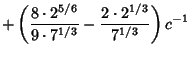
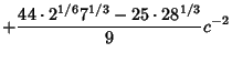
Saha and Strogatz (1995) give a simplified algebraic treatment which involves solving
| (24) |
| (25) | |||
| (26) | |||
| (27) |
| (28) | |||
| (29) | |||
| (30) |
| (31) |
| (32) |
|
|
(33) |
|
|
|
|
|
(34) |
The logistic equation has Correlation Exponent
![]() (Grassberger and Procaccia 1983), Capacity
Dimension 0.538 (Grassberger 1981), and Information Dimension 0.5170976 (Grassberger and Procaccia 1983).
(Grassberger and Procaccia 1983), Capacity
Dimension 0.538 (Grassberger 1981), and Information Dimension 0.5170976 (Grassberger and Procaccia 1983).
See also Bifurcation, Feigenbaum Constant, Logistic Distribution, Logistic Equation r=4, Logistic Growth Curve, Period Three Theorem, Quadratic Map
References
Bechhoeffer, J. ``The Birth of Period 3, Revisited.'' Math. Mag. 69, 115-118, 1996.
Bogomolny, A. ``Chaos Creation (There is Order in Chaos).''
http://www.cut-the-knot.com/blue/chaos.html.
Dickau, R. M. ``Bifurcation Diagram.''
http://forum.swarthmore.edu/advanced/robertd/bifurcation.html.
Gleick, J. Chaos: Making a New Science. New York: Penguin Books, pp. 69-80, 1988.
Gordon, W. B. ``Period Three Trajectories of the Logistic Map.'' Math. Mag. 69, 118-120, 1996.
Grassberger, P. ``On the Hausdorff Dimension of Fractal Attractors.'' J. Stat. Phys. 26, 173-179, 1981.
Grassberger, P. and Procaccia, I. ``Measuring the Strangeness of Strange Attractors.'' Physica D 9, 189-208, 1983.
Lauwerier, H. Fractals: Endlessly Repeated Geometrical Figures. Princeton, NJ: Princeton University Press, pp. 119-122, 1991.
May, R. M. ``Simple Mathematical Models with Very Complicated Dynamics.'' Nature 261, 459-467, 1976.
Peitgen, H.-O.; Jürgens, H.; and Saupe, D. Chaos and Fractals: New Frontiers of Science.
New York: Springer-Verlag, pp. 585-653, 1992.
Rasband, S. N. Chaotic Dynamics of Nonlinear Systems. New York: Wiley, p. 23, 1990.
Russell, D. A.; Hanson, J. D.; and Ott, E. ``Dimension of Strange Attractors.'' Phys. Rev. Let. 45, 1175-1178, 1980.
Saha, P. and Strogatz, S. H. ``The Birth of Period Three.'' Math. Mag. 68, 42-47, 1995.
Strogatz, S. H. Nonlinear Dynamics and Chaos. Reading, MA: Addison-Wesley, 1994.
Tabor, M. Chaos and Integrability in Nonlinear Dynamics: An Introduction. New York: Wiley, 1989.
Wagon, S. ``The Dynamics of the Quadratic Map.'' §4.4 in Mathematica in Action. New York: W. H. Freeman, pp. 117-140,
1991.
|
|
|
© 1996-9 Eric W. Weisstein