info prev up next book cdrom email home

Prolate Spheroidal Coordinates

\begin{figure}\begin{center}\BoxedEPSF{ProlateSpheroidalCoords.epsf scaled 900}\end{center}\end{figure}

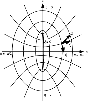
A system of Curvilinear Coordinates in which two sets of coordinate surfaces are obtained by revolving the curves of the Elliptic Cylindrical Coordinates about the x-Axis, which is relabeled the z-Axis. The third set of coordinates consists of planes passing through this axis.

$\displaystyle x$ $\textstyle =$ $\displaystyle a\sinh\xi\sin\eta\cos \phi$ (1)
$\displaystyle y$ $\textstyle =$ $\displaystyle a\sinh\xi\sin\eta\sin \phi$ (2)
$\displaystyle z$ $\textstyle =$ $\displaystyle a\cosh\xi\cos\eta,$ (3)

where $\xi \in [0, \infty)$, $\eta \in [0, \pi)$, and $\phi \in [0, 2\pi)$. Arfken (1970) uses $(u, v, \varphi)$ instead of $(\xi, \eta, z)$. The Scale Factors are
$\displaystyle h_\xi$ $\textstyle =$ $\displaystyle a \sqrt{\sinh^2\xi+\sin^2\eta}$ (4)
$\displaystyle h_\eta$ $\textstyle =$ $\displaystyle a \sqrt{\sinh^2\xi+\sin^2\eta}$ (5)
$\displaystyle h_\phi$ $\textstyle =$ $\displaystyle a \sinh\xi\sin\eta.$ (6)

The Laplacian is

$\nabla^2 f={1\over\sin\eta\sinh\xi(\sin^2\eta+\sinh^2\xi)}$
$ \times\left\{{{\partial\over\partial\xi}\left({\sin\eta\sinh\xi{\partial f\ove...
...i\sin\eta+\csc\eta\sinh\xi){\partial f\over\partial\phi}}\right]}\right\}.\quad$ (7)
$={1\over\sin^2\eta+\sinh^2\xi}\left[{(\csc^2\eta+\mathop{\rm csch}\nolimits ^2\...
...2}+\coth\xi{\partial f\over\partial\xi}+{\partial^2f\over\partial\xi^2}}\right]$ (8)


An alternate form useful for ``two-center'' problems is defined by

$\displaystyle \xi_1$ $\textstyle =$ $\displaystyle \cosh\xi$ (9)
$\displaystyle \xi_2$ $\textstyle =$ $\displaystyle \cos\eta$ (10)
$\displaystyle \xi_3$ $\textstyle =$ $\displaystyle \phi,$ (11)

where $\xi_1 \in [1,\infty]$, $\xi_2\in [-1,1]$, and $\xi_3\in [0,2\pi)$ (Abramowitz and Stegun 1972). In these coordinates,
$\displaystyle z$ $\textstyle =$ $\displaystyle a\xi_1\xi_2$ (12)
$\displaystyle x$ $\textstyle =$ $\displaystyle a\sqrt{({\xi_1}^2-1)(1-{\xi_2}^2)}\,\cos\xi_3$ (13)
$\displaystyle y$ $\textstyle =$ $\displaystyle a\sqrt{({\xi_1}^2-1)(1-{\xi_2}^2)}\,\sin\xi_3.$ (14)

In terms of the distances from the two Foci,
$\displaystyle \xi_1$ $\textstyle =$ $\displaystyle {r_1+r_2\over 2a}$ (15)
$\displaystyle \xi_2$ $\textstyle =$ $\displaystyle {r_1-r_2\over 2a}$ (16)
$\displaystyle 2a$ $\textstyle =$ $\displaystyle r_{12}.$ (17)

The Scale Factors are
$\displaystyle h_{\xi_1}$ $\textstyle =$ $\displaystyle a\sqrt{{\xi_1}^2-{\xi_2}^2\over{\xi_1}^2-1}$ (18)
$\displaystyle h_{\xi_2}$ $\textstyle =$ $\displaystyle a\sqrt{{\xi_1}^2-{\xi_2}^2\over 1-{\xi_2}^2}$ (19)
$\displaystyle h_{\xi_3}$ $\textstyle =$ $\displaystyle a\sqrt{({\xi_1}^2-1)(1-{\xi_2}^2)},$ (20)

and the Laplacian is

$\nabla^2 f = {1\over a^2}\left\{{{1\over{\xi_1}^2-{\xi_2}^2} {\partial \over \partial \xi_1}\left[{({\xi_1}^2-1) {\partial f\over \partial \xi_1}}\right]}\right.$
$ \mathop{+} \left.{{1\over{\xi_1}^2-{\xi_2}^2}{\partial\over\partial\xi_2}\left...
...({\xi_1}^2-1)(1-{\xi_2}^2)} {\partial^2 f\over\partial{\xi_3}^2}}\right\}.\quad$ (21)
The Helmholtz Differential Equation is separable in prolate spheroidal coordinates.

See also Helmholtz Differential Equation--Prolate Spheroidal Coordinates, Latitude, Longitude, Oblate Spheroidal Coordinates, Spherical Coordinates


References

Abramowitz, M. and Stegun, C. A. (Eds.). ``Definition of Prolate Spheroidal Coordinates.'' §21.2 in Handbook of Mathematical Functions with Formulas, Graphs, and Mathematical Tables, 9th printing. New York: Dover, p. 752, 1972.

Arfken, G. ``Prolate Spheroidal Coordinates ($u$, $v$, $\phi$).'' §2.10 in Mathematical Methods for Physicists, 2nd ed. Orlando, FL: Academic Press, pp. 103-107, 1970.

Morse, P. M. and Feshbach, H. Methods of Theoretical Physics, Part I. New York: McGraw-Hill, p. 661, 1953.


info prev up next book cdrom email home

© 1996-9 Eric W. Weisstein
1999-05-26