info prev up next book cdrom email home

Apodization Function

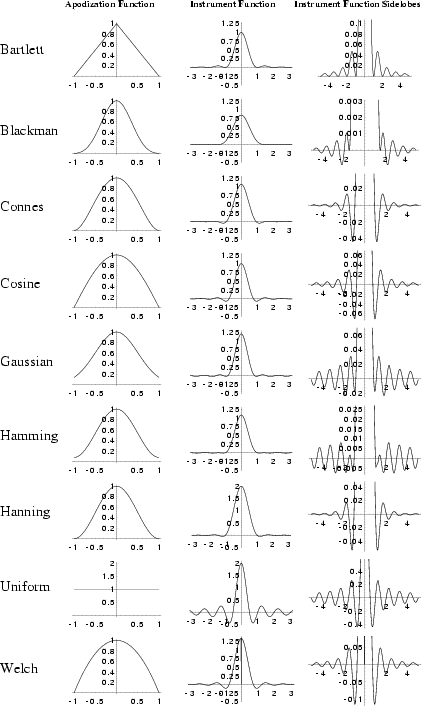
A function (also called a Tapering Function) used to bring an interferogram smoothly down to zero at the edges of the sampled region. This suppresses sidelobes which would otherwise be produced, but at the expense of widening the lines and therefore decreasing the resolution.


The following are apodization functions for symmetrical (2-sided) interferograms, together with the Instrument Functions (or Apparatus Functions) they produce and a blowup of the Instrument Function sidelobes. The Instrument Function $I(k)$ corresponding to a given apodization function $A(x)$ can be computed by taking the finite Fourier Cosine Transform,

\begin{displaymath}
I(k)=\int_{-a}^a \cos(2\pi kx)A(x)\,dx.
\end{displaymath} (1)

\begin{figure}\begin{center}\BoxedEPSF{InstrumentFunctions.epsf scaled 500}\end{center}\end{figure}

Type Apodization Function Instrument Function
Bartlett $1-{\vert x\vert\over a}$ $a\mathop{\rm sinc}\nolimits ^2(\pi ka)$
Blackman $B_A(x)$ $B_I(k)$
Connes $\left({1-{x^2\over a^2}}\right)^2$ $8a\sqrt{2\pi}\, {J_{5/2}(2\pi ka)\over (2\pi ka)^{5/2}}$
Cosine $\cos\left({\pi x\over 2a}\right)$ ${4a\cos(2\pi ak)\over \pi(1-16a^2 k^2)}$
Gaussian $e^{-x^2/(2\sigma^2)}$ $2\int_0^a \cos(2\pi kx)e^{-x^2/(2\sigma^2)}\,dx$
Hamming ${\it Hm}_A(x)$ ${\it Hm}_I(k)$
Hanning ${\it Hn}_A(x)$ ${\it Hn}_I(k)$
Uniform 1 $2a\mathop{\rm sinc}\nolimits \,(2\pi ka)$
Welch $1-{x^2\over a^2}$ $W_I(k)$

where


$\displaystyle B_A(x)$ $\textstyle =$ $\displaystyle 0.42+0.5\cos\left({\pi x\over a}\right)+0.08\cos\left({2\pi x\over a}\right)$ (2)
$\displaystyle B_I(k)$ $\textstyle =$ $\displaystyle {a(0.84-0.36 a^2k^2-2.17\times 10^{-19} a^4k^4)\mathop{\rm sinc}\nolimits (2\pi ak)\over (1-a^2k^2)(1-4a^2k^2)}$ (3)
      (4)
$\displaystyle {\it Hm}_A(x)$ $\textstyle =$ $\displaystyle 0.54+0.46\cos\left({\pi x\over a}\right)$ (5)
$\displaystyle {\it Hm}_I(k)$ $\textstyle =$ $\displaystyle {a(1.08-0.64a^2k^2)\mathop{\rm sinc}\nolimits (2\pi ak)\over 1-4a^2k^2}$ (6)
$\displaystyle {\it Hn}_A(x)$ $\textstyle =$ $\displaystyle \cos^2\left({\pi x\over 2a}\right)$ (7)
  $\textstyle =$ $\displaystyle {1\over 2}\left[{1+\cos\left({\pi x\over a}\right)}\right]$ (8)
$\displaystyle {\it Hn}_I(k)$ $\textstyle =$ $\displaystyle {a\mathop{\rm sinc}\nolimits \,(2\pi a k)\over 1-4a^2k^2}$ (9)
  $\textstyle =$ $\displaystyle a[\mathop{\rm sinc}\nolimits (2\pi ka)+{\textstyle{1\over 2}}\mat...
...s (2\pi ka-\pi)+{\textstyle{1\over 2}}\mathop{\rm sinc}\nolimits (2\pi ka+\pi)]$ (10)
$\displaystyle W_I(k)$ $\textstyle =$ $\displaystyle a 2\sqrt{2\pi}\, {J_{3/2}(2\pi ka)\over (2\pi ka)^{3/2}}$ (11)
  $\textstyle =$ $\displaystyle a{\sin(2\pi ka)-2\pi ak\cos(2\pi ak)\over 2a^3k^3\pi^3}.$ (12)

Type Instrument Function FWHM IF Peak ${\hbox{Peak $(-)$\ Sidelobe}\over \hbox{Peak}}$ ${\hbox{Peak $(+)$\ Sidelobe}\over \hbox{Peak}}$
Bartlett 1.77179 1 0.00000000 $0.0471904$
Blackman 2.29880 0.84 $-0.00106724$ 0.00124325
Connes 1.90416 ${\textstyle{16\over 15}}$ $-0.0411049$ $0.0128926$
Cosine 1.63941 ${\textstyle{4\over \pi}}$ $-0.0708048$ $0.0292720$
Gaussian -- 1 -- --
Hamming 1.81522 1.08 $-0.00689132$ 0.00734934
Hanning 2.00000 1 $-0.0267076$ 0.00843441
Uniform 1.20671 2 $-0.217234$ $0.128375$
Welch 1.59044 ${\textstyle{4\over 3}}$ $-0.0861713$ $0.356044$


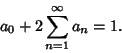
A general symmetric apodization function $A(x)$ can be written as a Fourier Series
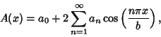
\begin{displaymath}
A(x)=a_0+2\sum_{n=1}^\infty a_n\cos\left({n\pi x\over b}\right),
\end{displaymath} (13)

where the Coefficients satisfy
\begin{displaymath}
a_0+2\sum_{n=1}^\infty a_n=1.
\end{displaymath} (14)

The corresponding apparatus function is
$I(t)\equiv \int_{-b}^b A(x)e^{-2\pi ikx}\,dx=2b\Bigl\{a_0\mathop{\rm sinc}\nolimits (2\pi kb)$
$ +\sum_{n=1}^\infty [\mathop{\rm sinc}\nolimits (2\pi kb+n\pi)+\mathop{\rm sinc}\nolimits (2\pi kb-n\pi)]\Bigr\}.\quad$ (15)
To obtain an Apodization Function with zero at $ka=3/4$, use
\begin{displaymath}
a_0\mathop{\rm sinc}\nolimits ({\textstyle{3\over 2}}\pi)+a_...
...\pi)+\mathop{\rm sinc}\nolimits ({\textstyle{1\over 2}}\pi)=0.
\end{displaymath} (16)

Plugging in (14),


\begin{displaymath}
-(1-2a_1){2\over 3\pi}+a_1\left({{2\over 5\pi}+{2\over\pi}}\...
...\textstyle{1\over 3}} (1-2a_1)+a_1({\textstyle{1\over 5}}+1)=0
\end{displaymath} (17)


\begin{displaymath}
a_1({\textstyle{6\over 5}}+{\textstyle{2\over 3}})={\textstyle{1\over 3}}
\end{displaymath} (18)


$\displaystyle a_1$ $\textstyle =$ $\displaystyle {{\textstyle{1\over 3}}\over{\textstyle{6\over 5}}+{\textstyle{2\over 3}}}={5\over 6\cdot 3+2\cdot 5} = {\textstyle{5\over 28}}$ (19)
$\displaystyle a_0$ $\textstyle =$ $\displaystyle 1-2a_1={28-2\cdot 5\over 28}={\textstyle{18\over 28}}={\textstyle{9\over 14}}.$ (20)

The Hamming Function is close to the requirement that the Apparatus Function goes to 0 at $ka=5/4$, giving
$\displaystyle a_0$ $\textstyle =$ $\displaystyle {\textstyle{25\over 46}}\approx 0.5435$ (21)
$\displaystyle a_1$ $\textstyle =$ $\displaystyle {\textstyle{21\over 92}}\approx 0.2283.$ (22)

The Blackman Function is chosen so that the Apparatus Function goes to 0 at $ka=5/4$ and 9/4, giving
$\displaystyle a_0$ $\textstyle =$ $\displaystyle {\textstyle{3969\over 9304}}\approx 0.4266$ (23)
$\displaystyle a_1$ $\textstyle =$ $\displaystyle {\textstyle{1155\over 4652}}\approx 0.2483$ (24)
$\displaystyle a_2$ $\textstyle =$ $\displaystyle {\textstyle{715\over 18608}}\approx 0.0384.$ (25)

See also Bartlett Function, Blackman Function, Connes Function, Cosine Apodization Function, Full Width at Half Maximum, Gaussian Function, Hamming Function, Hann Function, Hanning Function, Mertz Apodization Function, Parzen Apodization Function, Uniform Apodization Function, Welch Apodization Function


References

Ball, J. A. ``The Spectral Resolution in a Correlator System'' §4.3.5 in Methods of Experimental Physics 12C (Ed. M. L. Meeks). New York: Academic Press, pp. 55-57, 1976.

Blackman, R. B. and Tukey, J. W. ``Particular Pairs of Windows.'' In The Measurement of Power Spectra, From the Point of View of Communications Engineering. New York: Dover, pp. 95-101, 1959.

Brault, J. W. ``Fourier Transform Spectrometry.'' In High Resolution in Astronomy: 15th Advanced Course of the Swiss Society of Astronomy and Astrophysics (Ed. A. Benz, M. Huber, and M. Mayor). Geneva Observatory, Sauverny, Switzerland, pp. 31-32, 1985.

Harris, F. J. ``On the Use of Windows for Harmonic Analysis with the Discrete Fourier Transform.'' Proc. IEEE 66, 51-83, 1978.

Norton, R. H. and Beer, R. ``New Apodizing Functions for Fourier Spectroscopy.'' J. Opt. Soc. Amer. 66, 259-264, 1976.

Press, W. H.; Flannery, B. P.; Teukolsky, S. A.; and Vetterling, W. T. Numerical Recipes in FORTRAN: The Art of Scientific Computing, 2nd ed. Cambridge, England: Cambridge University Press, pp. 547-548, 1992.

Schnopper, H. W. and Thompson, R. I. ``Fourier Spectrometers.'' In Methods of Experimental Physics 12A (Ed. M. L. Meeks). New York: Academic Press, pp. 491-529, 1974.


info prev up next book cdrom email home

© 1996-9 Eric W. Weisstein
1999-05-25