info prev up next book cdrom email home

Geometric Distribution

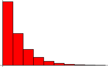
\begin{figure}\begin{center}\BoxedEPSF{GeometricDistribution.epsf}\end{center}\end{figure}

A distribution such that

\begin{displaymath}
P(n) = q^{n-1}p = p(1-p)^{n-1},
\end{displaymath} (1)

where $q\equiv 1-p$ and for $n = 1,$ 2, .... The distribution is normalized since
\begin{displaymath}
\sum_{n=1}^\infty P(n) = \sum_{n=1}^\infty q^{n-1}p
= p\sum_{n=0}^\infty q^n = {p\over 1-q} = {p\over p} = 1.
\end{displaymath} (2)

The Moment-Generating Function is
\begin{displaymath}
\phi(t)=p[1-(1-p)e^{it}]^{-1},
\end{displaymath} (3)

or
$\displaystyle M(t)$ $\textstyle =$ $\displaystyle \left\langle{e^{tn}}\right\rangle{} = \sum_{n=1}^\infty e^{tn} pq^{n-1} =p\sum_{n=0}^\infty e^{t(n+1)}q^n$  
  $\textstyle =$ $\displaystyle pe^t\sum_{n=0}^\infty (e^tq)^n={pe^t\over 1-e^tq}$ (4)
$\displaystyle M'(t)$ $\textstyle =$ $\displaystyle p\left[{(1-e^tq)e^t-e^t(-e^tq)\over (1-e^tq)^2}\right]$  
  $\textstyle =$ $\displaystyle {p(e^t-qe^{2t}+qe^{2t})\over (1-e^tq)^2}= {pe^t\over (1-e^tq)^2}$ (5)
$\displaystyle M''(t)$ $\textstyle =$ $\displaystyle p {(1-e^tq)^2e^t-e^t 2(1-e^tq)(-e^tq)\over (1-e^tq)^4}$  
  $\textstyle =$ $\displaystyle p {(1-2e^tq+e^{2t}q^2)e^t+2qe^{2t}(1-e^tq)\over (1-e^tq)^4}$  
  $\textstyle =$ $\displaystyle p {e^t-2e^{2t}q+e^{3t}q^2+2qe^{2t}-2q^2e^{3t}\over (1-e^tq)^4}$  
  $\textstyle =$ $\displaystyle p{e^t-q^2e^{3t}\over (1-e^tq)^4}= {pe^t(1-q^2e^{2t})\over (1-e^tq)^4}$  
  $\textstyle =$ $\displaystyle {pe^t(1+qe^t)\over(1-e^tq)^3}$ (6)
$\displaystyle M'''(t)$ $\textstyle =$ $\displaystyle {pe^t[1+4e^t(1-p)+e^{2t}(1-p)^2]\over (1-e^t+e^tp)^4}.$ (7)

Therefore,
$\displaystyle M'(0)$ $\textstyle =$ $\displaystyle \mu'_1 =\mu = {p\over (1-q)^2} = {p\over p^2} = {1\over p}$ (8)
$\displaystyle M''(0)$ $\textstyle =$ $\displaystyle \mu'_2 = {p(1+q)\over (1+q)^3} = {p(2-p)\over p^3}= {2-p\over p^2}$ (9)
$\displaystyle M'''(0)$ $\textstyle =$ $\displaystyle \mu'_3 = {(6-6p+p^2)\over p^3}$ (10)
$\displaystyle M^{(4)}(0)$ $\textstyle =$ $\displaystyle \mu'_4 = {(p-2)(-p^2+12p-12)\over p^4},$ (11)

and


$\displaystyle \mu_2$ $\textstyle \equiv$ $\displaystyle \mu_2'-(\mu_1')^2 = \left({{2\over p^2}-{1\over p}}\right)-{1\over p^2}= {1-p\over p^2}$  
  $\textstyle =$ $\displaystyle {q\over p^2}$ (12)
$\displaystyle \mu_3$ $\textstyle \equiv$ $\displaystyle \mu_3'-3\mu_2'\mu_1'+2(\mu_1')^3$  
  $\textstyle =$ $\displaystyle {6-6p+p^2\over p^3}-3{2-p\over p^2}{1\over p}+2\left({1\over p}\right)^3$  
  $\textstyle =$ $\displaystyle {6-6p+p^2-3(2-p)+2\over p^3}$  
  $\textstyle =$ $\displaystyle {(p-1)(p-2)\over p^3}$ (13)
$\displaystyle \mu_4$ $\textstyle \equiv$ $\displaystyle \mu_4'-4\mu_3'\mu_1'+6\mu_2'(\mu_1')^2-3(\mu_1')^4$  
  $\textstyle =$ $\displaystyle {(p-2)(-p^2+12p-12)\over p^4}-4 {6-6p+p^2\over p^3}{1\over p}+6 {2-p\over p^2}\left({1\over p}\right)^2-3\left({1\over p}\right)^4$  
  $\textstyle =$ $\displaystyle {(p-1)(-p^2+9p-9)\over p^4},$ (14)

so the Mean, Variance, Skewness, and Kurtosis are given by
$\displaystyle \mu$ $\textstyle \equiv$ $\displaystyle \mu'_1={1\over p}$ (15)
$\displaystyle \sigma^2$ $\textstyle =$ $\displaystyle \mu_2={q\over p^2}$ (16)
$\displaystyle \gamma_1$ $\textstyle =$ $\displaystyle {\mu_3\over \sigma^3} ={(p-1)(p-2)\over p^3} \left({p^2\over 1-p}\right)^{3/2}$  
  $\textstyle =$ $\displaystyle {(p-1)(p-2)\over (1-p)\sqrt{1-p}} = {2-p\over \sqrt{1-p}} = {2-p\over\sqrt{q}}$ (17)
$\displaystyle \gamma_2$ $\textstyle =$ $\displaystyle {\mu_4\over\sigma^4}-3= {(p-1)(-p^2+9p-9)\over p^4{(1-p)^2\over p^4}}-3$  
  $\textstyle =$ $\displaystyle {-9+9p-p^2\over (p-1)}-3$  
  $\textstyle =$ $\displaystyle {p^2-6p+6\over 1-p}.$ (18)

In fact, the moments of the distribution are given analytically in terms of the Polylogarithm function,
\begin{displaymath}
\mu_k'\equiv \sum_{n=1}^\infty P(n)n^k = \sum_{n=1}^\infty p...
...)^{n-1} n^k = {p\mathop{\rm Li}\nolimits _{-k}(1-p)\over 1-p}.
\end{displaymath} (19)

For the case $p=1/2$ (corresponding to the distribution of the number of Coin Tosses needed to win in the Saint Petersburg Paradox) this formula immediately gives
$\displaystyle \mu'_1$ $\textstyle =$ $\displaystyle 2$ (20)
$\displaystyle {\mu'}_2$ $\textstyle =$ $\displaystyle 6$ (21)
$\displaystyle \mu'_3$ $\textstyle =$ $\displaystyle 26$ (22)
$\displaystyle \mu'_4$ $\textstyle =$ $\displaystyle 150,$ (23)

so the Mean, Variance, Skewness, and Kurtosis in this case are
$\displaystyle \mu$ $\textstyle =$ $\displaystyle 2$ (24)
$\displaystyle \sigma^2$ $\textstyle =$ $\displaystyle 2$ (25)
$\displaystyle \gamma_1$ $\textstyle =$ $\displaystyle {\textstyle{3\over 2}}\sqrt{2}$ (26)
$\displaystyle \gamma_2$ $\textstyle =$ $\displaystyle {\textstyle{13\over 2}}.$ (27)


The first Cumulant of the geometric distribution is

\begin{displaymath}
\kappa_1={1-p\over p},
\end{displaymath} (28)

and subsequent Cumulants are given by the Recurrence Relation
\begin{displaymath}
\kappa_{r+1}=(1-p){d\kappa_r\over dp}.
\end{displaymath} (29)

See also Saint Petersburg Paradox


References

Beyer, W. H. CRC Standard Mathematical Tables, 28th ed. Boca Raton, FL: CRC Press, pp. 531-532, 1987.

Spiegel, M. R. Theory and Problems of Probability and Statistics. New York: McGraw-Hill, p. 118, 1992.


info prev up next book cdrom email home

© 1996-9 Eric W. Weisstein
1999-05-25