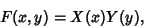
Given a first-order Ordinary Differential Equation
 |
(1) |
if  can be expressed using Separation of Variables as
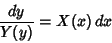
 |
(2) |
then the equation can be expressed as
 |
(3) |
and the equation can be solved by integrating both sides to obtain
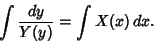 |
(4) |
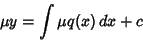
Any first-order ODE of the form
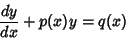 |
(5) |
can be solved by finding an Integrating Factor  such that
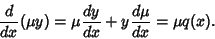 |
(6) |
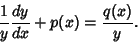
Dividing through by  yields
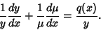 |
(7) |
However, this condition enables us to explicitly determine the appropriate  for arbitrary
  and
and  . To accomplish
this, take
. To accomplish
this, take
 |
(8) |
in the above equation, from which we recover the original equation (5), as required, in the form
 |
(9) |
But we can integrate both sides of (8) to obtain
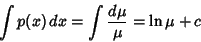 |
(10) |
 |
(11) |
Now integrating both sides of (6) gives
 |
(12) |
(with now a known function), which can be solved for  to obtain
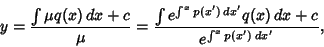 |
(13) |
where  is an arbitrary constant of integration.
Given an  th-order linear ODE with constant Coefficients
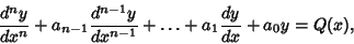 |
(14) |
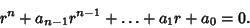
first solve the characteristic equation obtained by writing
 |
(15) |
and setting  to obtain the Complex Roots.
 |
(16) |
 |
(17) |
Factoring gives the Roots  ,
,
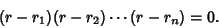 |
(18) |
For a nonrepeated Real Root  , the corresponding solution is
 |
(19) |
If a Real Root is repeated  times, the solutions are degenerate and the linearly
independent solutions are
times, the solutions are degenerate and the linearly
independent solutions are
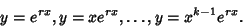 |
(20) |
Complex Roots always come in Complex Conjugate pairs,
 . For nonrepeated
Complex Roots, the solutions are
. For nonrepeated
Complex Roots, the solutions are
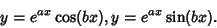 |
(21) |
If the Complex Roots are repeated times, the linearly independent solutions
are
 |
(22) |
Linearly combining solutions of the appropriate types with arbitrary multiplicative constants then gives the complete
solution. If initial conditions are specified, the constants can be explicitly determined. For example, consider the
sixth-order linear ODE
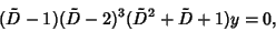 |
(23) |
which has the characteristic equation
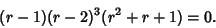 |
(24) |
The roots are 1, 2 (three times), and
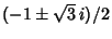 , so the solution is
 |
(25) |
If the original equation is nonhomogeneous ( ), now find the particular solution
  by the method of
Variation of Parameters. The general solution is then
by the method of
Variation of Parameters. The general solution is then
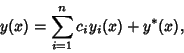 |
(26) |
where the solutions to the linear equations are  ,
,  , ...,
  , and
, and  is the particular
solution.
is the particular
solution.
See also Integrating Factor, Ordinary Differential Equation--First-Order Exact, Separation of Variables, Variation of Parameters
References
Arfken, G. Mathematical Methods for Physicists, 3rd ed. Orlando, FL: Academic Press, pp. 440-445, 1985.
© 1996-9 Eric W. Weisstein
1999-05-26