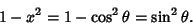
The second-order Ordinary Differential Equation
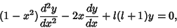 |
(1) |
which can be rewritten
![\begin{displaymath}
{d\over dx} \left[{(1-x^2) {dy\over dx}}\right]+ l(l+1) y = 0.
\end{displaymath}](l1_1221.gif) |
(2) |
The above form is a special case of the associated Legendre differential equation with  . The Legendre differential
equation has Regular Singular Points at
. The Legendre differential
equation has Regular Singular Points at  , 1, and
  . It can be solved using a
series expansion,
. It can be solved using a
series expansion,
Plugging in,
 |
(6) |

|
|

|
(7) |
|
|
|
(8) |

|
|
|
|
(9) |
![\begin{displaymath}
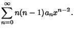
\sum_{n=0}^\infty \{(n+1)(n+2)a_{n+2}+[-n(n-1)-2n+l(l+1)]a_n\} = 0,
\end{displaymath}](l1_1235.gif) |
(10) |
so each term must vanish and
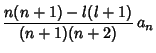
![\begin{displaymath}
(n+1)(n+2)a_{n+2}-n(n+1)+l(l+1)]a_n = 0
\end{displaymath}](l1_1236.gif) |
(11) |
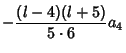
Therefore,
so the Even solution is
![\begin{displaymath}
y_1(x) = 1+\sum_{n=1}^\infty (-1)^n {[(l-2n+2)\cdots(l-2)l][(l+1)(l+3)\cdots (l+2n-1)] \over (2n)!} x^{2n}.
\end{displaymath}](l1_1248.gif) |
(16) |
Similarly, the Odd solution is
![\begin{displaymath}
y_2(x)= x+\sum_{n=1}^\infty(-1)^n{[(l-2n+1)\cdots(l-3)(l-1)][(l+2)(l+4)\cdots(l+2n)\over (2n+1)!}x^{2m+1}.
\end{displaymath}](l1_1249.gif) |
(17) |
If  is an Even Integer, the series
  reduces to a Polynomial of degree with only Even
Powers of
reduces to a Polynomial of degree with only Even
Powers of  and the series
  diverges. If is an Odd Integer, the series reduces
to a Polynomial of degree with only Odd Powers of and the series diverges. The
general solution for an Integer is given by the Legendre Polynomials
diverges. If is an Odd Integer, the series reduces
to a Polynomial of degree with only Odd Powers of and the series diverges. The
general solution for an Integer is given by the Legendre Polynomials
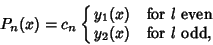 |
(18) |
where  is chosen so that
  . If the variable is replaced by
  , then the Legendre
differential equation becomes
, then the Legendre
differential equation becomes
 |
(19) |
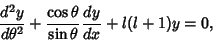
as is derived for the associated Legendre differential equation with .
The associated Legendre differential equation is
![\begin{displaymath}
{d\over dx} \left[{(1-x^2) {dy\over dx}}\right]+ \left[{l(l+1) - {m^2\over 1-x^2}}\right]y = 0
\end{displaymath}](l1_1258.gif) |
(20) |
![\begin{displaymath}
(1-x^2) {d^2y\over dx^2} - 2x {dy\over dx}+\left[{l(l+1) - {m^2\over 1-x^2}}\right]y = 0.
\end{displaymath}](l1_1259.gif) |
(21) |
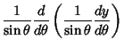
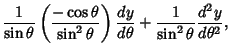
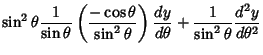
The solutions to this equation are called the associated Legendre polynomials. Writing
 , first establish
the identities
, first establish
the identities
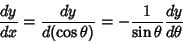 |
(22) |
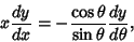 |
(23) |
and
 |
(25) |
Therefore,
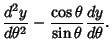
Plugging (22) into (26) and the result back into (21) gives
![\begin{displaymath}
\left({{d^2y\over d\theta^2}-{\cos\theta\over\sin\theta} {dy...
...r d\theta}+\left[{l(l+1) - {m^2\over\sin^2\theta}}\right]y = 0
\end{displaymath}](l1_1270.gif) |
(27) |
![\begin{displaymath}
{d^2y\over d\theta^2} + {\cos\theta\over\sin\theta} {dy\over dx} + \left[{l(l+1) - {m^2\over\sin^2\theta}}\right]y = 0.
\end{displaymath}](l1_1271.gif) |
(28) |
References
Abramowitz, M. and Stegun, C. A. (Eds.).
Handbook of Mathematical Functions with Formulas, Graphs, and Mathematical Tables, 9th printing.
New York: Dover, p. 332, 1972.
© 1996-9 Eric W. Weisstein
1999-05-26


\over (n+1)(n+2)}\, a_n.$](l1_1239.gif)

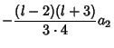
![$\displaystyle (-1)^2 {[(l-2)l][(l+1)(l+3)]\over 1\cdot 2\cdot 3\cdot 4 } a_0$](l1_1244.gif)
![$\displaystyle (-1)^3 {[(l-4)(l-2)l][(l+1)(l+3)(l+5)]\over 1\cdot 2\cdot 3\cdot 4\cdot 5\cdot 6} a_0,$](l1_1247.gif)