info prev up next book cdrom email home

Mercator Projection

\begin{figure}\begin{center}\BoxedEPSF{maps/merc.epsf scaled 500}\end{center}\end{figure}

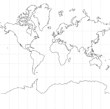
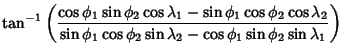
The following equations place the x-Axis of the projection on the equator and the y-Axis at Longitude $\lambda_0$, where $\lambda$ is the Longitude and $\phi$ is the Latitude.

$\displaystyle x$ $\textstyle =$ $\displaystyle \lambda-\lambda_0$ (1)
$\displaystyle y$ $\textstyle =$ $\displaystyle \ln[\tan({\textstyle{1\over 4}}\pi+{\textstyle{1\over 2}}\phi)]$ (2)
  $\textstyle =$ $\displaystyle {\textstyle{1\over 2}}\ln\left({1+\sin\phi\over 1-\sin\phi}\right)$ (3)
  $\textstyle =$ $\displaystyle \sinh^{-1}(\tan\phi)$ (4)
  $\textstyle =$ $\displaystyle \tanh^{-1}(\sin\phi)$ (5)
  $\textstyle =$ $\displaystyle \ln(\tan\phi+\sec\phi).$ (6)

The inverse Formulas are
$\displaystyle \phi$ $\textstyle =$ $\displaystyle 2\tan^{-1}(e^y)=\tan^{-1}(\sinh y)=\mathop{\rm gd}\nolimits y$ (7)
$\displaystyle \lambda$ $\textstyle =$ $\displaystyle x+\lambda_0,$ (8)

where $\mathop{\rm gd}\nolimits y$ is the Gudermannian Function. Loxodromes are straight lines and Great Circles are curved.


\begin{figure}\begin{center}\BoxedEPSF{maps/mobl.epsf scaled 600}\end{center}\end{figure}

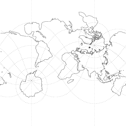
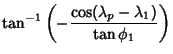
An oblique form of the Mercator projection is illustrated above. It has equations

$\displaystyle x$ $\textstyle =$ $\displaystyle {\tan^{-1}[\tan\phi\cos\phi_p+\sin\phi_p\sin(\lambda-\lambda_0)]\over\cos(\lambda-\lambda_0)}$ (9)
$\displaystyle y$ $\textstyle =$ $\displaystyle {\textstyle{1\over 2}}\ln\left({1+A\over 1-A}\right)= \tanh^{-1} A,$ (10)

where
$\displaystyle \lambda_p$ $\textstyle =$ $\displaystyle \tan^{-1}\left({\cos\phi_1\sin\phi_2\cos\lambda_1-\sin\phi_1\cos\...
...ver
\sin\phi_1\cos\phi_2\sin\lambda_2-\cos\phi_1\sin\phi_2\sin\lambda_1}\right)$  
      (11)
$\displaystyle \phi_p$ $\textstyle =$ $\displaystyle \tan^{-1}\left({-{\cos(\lambda_p-\lambda_1)\over\tan\phi_1}}\right)$ (12)
$\displaystyle A$ $\textstyle =$ $\displaystyle \sin\phi_p\sin\phi-\cos\phi_p\cos\phi\sin(\lambda-\lambda_0).$ (13)

The inverse Formulas are
$\displaystyle \phi$ $\textstyle =$ $\displaystyle \sin^{-1}\left({\sin\phi_p\tanh y+{\cos\phi_p\sin x\over\cosh y}}\right)$ (14)
$\displaystyle \lambda$ $\textstyle =$ $\displaystyle \lambda_0+\tan^{-1}\left({\sin\phi_p\sin x-\cos\phi_p\sinh y\over \cos x}\right).$ (15)


\begin{figure}\begin{center}\BoxedEPSF{maps/mtra.epsf scaled 400}\end{center}\end{figure}

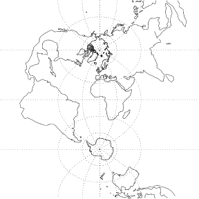
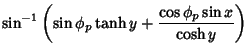
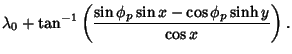
There is also a transverse form of the Mercator projection, illustrated above. It is given by the equations

$\displaystyle x$ $\textstyle =$ $\displaystyle {\textstyle{1\over 2}}\ln\left({1+B\over 1-B}\right)=\tanh^{-1} B$ (16)
$\displaystyle y$ $\textstyle =$ $\displaystyle \tan^{-1}\left[{\tan\phi\over \cos(\lambda-\lambda_0)}\right]-\phi_0$ (17)
$\displaystyle \phi$ $\textstyle =$ $\displaystyle \sin^{-1}\left({\sin D\over\cosh x}\right)$ (18)
$\displaystyle \lambda$ $\textstyle =$ $\displaystyle \lambda_0+\tan^{-1}\left({\sinh x\over\cos D}\right),$ (19)

where
$\displaystyle B$ $\textstyle \equiv$ $\displaystyle \cos\phi\sin(\lambda-\lambda_0)$ (20)
$\displaystyle D$ $\textstyle \equiv$ $\displaystyle y+\phi_0.$ (21)


Finally, the ``universal transverse Mercator projection'' is a Map Projection which maps the Sphere into 60 zones of 6° each, with each zone mapped by a transverse Mercator projection with central Meridian in the center of the zone. The zones extend from 80° S to 84° N (Dana).

See also Gudermannian Function, Spherical Spiral


References

Dana, P. H. ``Map Projections.'' http://www.utexas.edu/depts/grg/gcraft/notes/mapproj/mapproj.html.

Snyder, J. P. Map Projections--A Working Manual. U. S. Geological Survey Professional Paper 1395. Washington, DC: U. S. Government Printing Office, pp. 38-75, 1987.


info prev up next book cdrom email home

© 1996-9 Eric W. Weisstein
1999-05-26