Given a function  of a variable
  tabulated at
  values
  , ...,
  , assume the function is
of known analytic form depending on
  parameters
 , and consider the overdetermined set
of
  equations
We desire to solve these equations to obtain the values  , ...,
  which best satisfy this system
of equations. Pick an initial guess for the
  and then define
 |
(3) |
Now obtain a linearized estimate for the changes  needed to reduce
  to 0,
to 0,
 |
(4) |
for  , ...,
  . This can be written in component form as
 |
(5) |
where
 is the
  Matrix
![\begin{displaymath}
A_{ij}=\left[{\matrix{
\left.{\partial f\over\partial\lambda...
...}\right\vert _{x_m,\boldsymbol{\lambda}} & \cdots\cr}}\right].
\end{displaymath}](n_763.gif) |
(6) |
In more concise Matrix form,
 |
(7) |
where
 and
and
 are
are  -Vectors. Applying the Matrix Transpose of
 to both
sides gives
 |
(8) |
Defining
in terms of the known quantities
 and
and
 then gives the Matrix Equation
 |
(11) |
which can be solved for
 using standard matrix techniques such as Gaussian Elimination. This offset is
then applied to
 and a new
  is calculated. By iteratively applying this procedure until the elements of
 become smaller than some prescribed limit, a solution is obtained. Note that the procedure may not converge
very well for some functions and also that convergence is often greatly improved by picking initial values close to the
best-fit value. The sum of square residuals is given by
 after the final iteration.
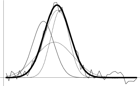
An example of a nonlinear least squares fit to a noisy Gaussian Function
 |
(12) |
is shown above, where the thin solid curve is the initial guess, the dotted curves are intermediate iterations, and the heavy
solid curve is the fit to which the solution converges. The actual parameters are
 , the initial
guess was (0.8, 15, 4), and the converged values are (1.03105, 20.1369, 4.86022), with
  . The Partial
Derivatives used to construct the matrix
 are
are
The technique could obviously be generalized to multiple Gaussians, to include slopes, etc., although the
convergence properties generally worsen as the number of free parameters is increased.
An analogous technique can be used to solve an overdetermined set of equations. This problem might, for example, arise
when solving for the best-fit Euler Angles corresponding to a noisy Rotation Matrix, in which case there are
three unknown angles, but nine correlated matrix elements. In such a case, write the  different functions as
 for
for  , ...,
  , call their actual values
  , and define
![\begin{displaymath}
{\hbox{\sf A}}=\left[{\matrix{
\left.{\partial f_1\over\par...
...al\lambda_n}\right\vert _{\boldsymbol{\lambda}_i}\cr}}\right],
\end{displaymath}](n_788.gif) |
(16) |
and
 |
(17) |
where
 are the numerical values obtained after the
  th iteration. Again, set up the equations as
 |
(18) |
and proceed exactly as before.
See also Least Squares Fitting, Linear Regression, Moore-Penrose Generalized Matrix Inverse
© 1996-9 Eric W. Weisstein
1999-05-25
![]() of a variable
of a variable ![]() tabulated at
tabulated at ![]() values
values ![]() , ...,
, ..., ![]() , assume the function is
of known analytic form depending on
, assume the function is
of known analytic form depending on ![]() parameters
parameters
![]() , and consider the overdetermined set
of
, and consider the overdetermined set
of ![]() equations
equations

![\begin{displaymath}
A_{ij}=\left[{\matrix{
\left.{\partial f\over\partial\lambda...
...}\right\vert _{x_m,\boldsymbol{\lambda}} & \cdots\cr}}\right].
\end{displaymath}](n_763.gif)


![]() different functions as
different functions as
![]() for
for ![]() , ...,
, ..., ![]() , call their actual values
, call their actual values ![]() , and define
, and define
![\begin{displaymath}
{\hbox{\sf A}}=\left[{\matrix{
\left.{\partial f_1\over\par...
...al\lambda_n}\right\vert _{\boldsymbol{\lambda}_i}\cr}}\right],
\end{displaymath}](n_788.gif)