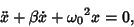
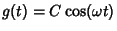
Simple harmonic motion refers to the periodic sinusoidal oscillation of an object or quantity. Simple harmonic motion is
executed by any quantity obeying the Differential Equation
 |
(1) |
where  denotes the second Derivative of
  with respect to
  , and
, and  is the angular frequency of oscillation. This Ordinary Differential Equation
has an irregular Singularity at
is the angular frequency of oscillation. This Ordinary Differential Equation
has an irregular Singularity at  . The general solution
is
. The general solution
is
where the two constants  and
and  (or
(or  and
and  ) are determined from the initial conditions.
Many physical systems undergoing small displacements, including any objects obeying
Hooke's law,  exhibit simple harmonic motion. This equation arises, for example,
in the analysis of the flow of
current in an electronic CL circuit (which contains a
capacitor and an inductor ). If a damping force such as
Friction is present, an additional term
exhibit simple harmonic motion. This equation arises, for example,
in the analysis of the flow of
current in an electronic CL circuit (which contains a
capacitor and an inductor ). If a damping force such as
Friction is present, an additional term  must be added to the Differential Equation and
motion dies out over time.
must be added to the Differential Equation and
motion dies out over time.
Adding a damping force proportional to  , the first derivative of with
respect to time, the equation of motion for damped simple harmonic motion is
, the first derivative of with
respect to time, the equation of motion for damped simple harmonic motion is
 |
(4) |
where  is the damping constant. This equation arises, for example, in the analysis of the flow of
current in an electronic CLR circuit, (which contains a
capacitor, an inductor, and a
resistor ). This Ordinary Differential Equation can be solved by looking for trial solutions
of the form
is the damping constant. This equation arises, for example, in the analysis of the flow of
current in an electronic CLR circuit, (which contains a
capacitor, an inductor, and a
resistor ). This Ordinary Differential Equation can be solved by looking for trial solutions
of the form  . Plugging this into (4) gives
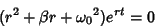 |
(5) |
 |
(6) |
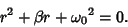
This is a Quadratic Equation with solutions
 |
(7) |
There are therefore three solution regimes depending on the Sign of the quantity inside the Square Root,
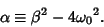 |
(8) |
The three regimes are
- 1.
 is Positive: overdamped,
- 2.
 is Zero: critically damped,
- 3.
 is Negative: underdamped.
If a periodic (sinusoidal) forcing term is added at angular frequency  , the same three solution regimes are again
obtained. Surprisingly, the resulting motion is still periodic (after an initial transient response, corresponding to the
solution to the unforced case, has died out), but it has an amplitude different from the forcing amplitude.
, the same three solution regimes are again
obtained. Surprisingly, the resulting motion is still periodic (after an initial transient response, corresponding to the
solution to the unforced case, has died out), but it has an amplitude different from the forcing amplitude.
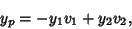
The ``particular'' solution  to the forced second-order nonhomogeneous Ordinary Differential Equation
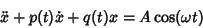 |
(9) |
due to forcing is given by the equation
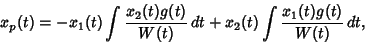 |
(10) |
where  and
and  are the homogeneous solutions to the unforced equation
 |
(11) |
and  is the Wronskian of these two functions. Once the sinusoidal case of forcing is solved, it can
be generalized to any periodic function by expressing the periodic function in a Fourier Series.
is the Wronskian of these two functions. Once the sinusoidal case of forcing is solved, it can
be generalized to any periodic function by expressing the periodic function in a Fourier Series.
Critical damping is a special case of damped simple harmonic motion in which
 |
(12) |
so
 |
(13) |
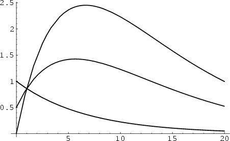
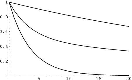
The above plot shows an underdamped simple harmonic oscillator with  ,
,  . The solid curve is for
 , the dot-dashed for (0, 1), and the dotted for (1/2, 1/2). In this case, so the solutions of the
form satisfy
, the dot-dashed for (0, 1), and the dotted for (1/2, 1/2). In this case, so the solutions of the
form satisfy
 |
(14) |
One of the solutions is therefore
 |
(15) |
In order to find the other linearly independent solution, we can make use of the identity
![\begin{displaymath}
x_2(t)=x_1(t)\int {e^{-\int p(t)\,dt}\over [x_1(t)]^2}\,dt.
\end{displaymath}](s1_1184.gif) |
(16) |
Since we have
 ,
,
 simplifies to
 . Equation (16) therefore
becomes
. Equation (16) therefore
becomes
![\begin{displaymath}
x_2(t) = e^{-{\omega_0}t} \int{e^{-2{\omega_0}t}\over [e^{-{...
...0}t}]^2}\, dt = e^{-{\omega_0}t} \int dt = t e^{-{\omega_0}t}.
\end{displaymath}](s1_1188.gif) |
(17) |
The general solution is therefore
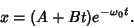 |
(18) |
In terms of the constants and , the initial values are
so
For sinusoidally forced simple harmonic motion with critical damping, the equation of motion is
 |
(23) |
and the Wronskian is
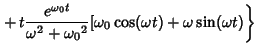
Plugging this into the equation for the particular solution gives
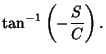
In order to put this in the desired form, note that we want to equate
This means
so
Plugging in,
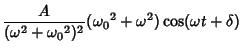
The solution in the requested form is therefore
where  is defined by (32).
Overdamped simple harmonic motion occurs when
 |
(34) |
so
 |
(35) |
The above plot shows an overdamped simple harmonic oscillator with ,  . The solid curve
is for , the dot-dashed for (0, 1), and the dotted for (1/2, 1/2). The solutions are
. The solid curve
is for , the dot-dashed for (0, 1), and the dotted for (1/2, 1/2). The solutions are
where
 |
(38) |
The general solution is therefore
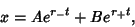 |
(39) |
where and are constants. The initial values are
so
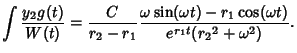
For a cosinusoidally forced overdamped oscillator with forcing function
 , the particular solutions
are
, the particular solutions
are
where
These give the identities
and
The Wronskian is
The particular solution is
 |
(52) |
where
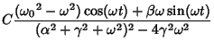
Therefore,
where
 |
(56) |
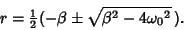
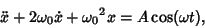
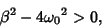
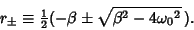
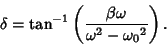
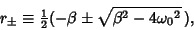
Underdamped simple harmonic motion occurs when
 |
(57) |
so
 |
(58) |
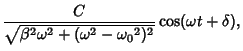
The above plot shows an underdamped simple harmonic oscillator with ,  . The solid curve
is for , the dot-dashed for (0, 1), and the dotted for (1/2, 1/2). Define
. The solid curve
is for , the dot-dashed for (0, 1), and the dotted for (1/2, 1/2). Define
 |
(59) |
then solutions satisfy
 |
(60) |
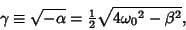
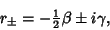
where
 |
(61) |
and are of the form
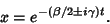 |
(62) |
Using the Euler Formula
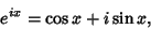 |
(63) |
this can be rewritten
![\begin{displaymath}
x = e^{-(\beta/2)t} \left[{\cos\left({\gamma t}\right)\pm i \sin\left({\gamma t}\right)}\right].
\end{displaymath}](s1_1275.gif) |
(64) |
We are interested in the real solutions. Since we are dealing here with a linear homogeneous ODE, linear
sums of Linearly Independent solutions are also solutions. Since we have a sum of such solutions in (64), it
follows that the Imaginary and Real Parts separately satisfy the ODE and are therefore the solutions we seek. The
constant in front of the sine term is arbitrary, so we can identify the solutions as
so the general solution is
![\begin{displaymath}
x= e^{-(\beta/2)t}[A\cos(\gamma t)+B\sin(\gamma t)].
\end{displaymath}](s1_1278.gif) |
(67) |
The initial values are
so and can be expressed in terms of the initial conditions by
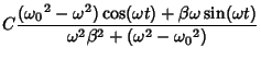
For a cosinusoidally forced underdamped oscillator with forcing function
, use
to obtain
The particular solutions are
The Wronskian is
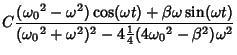
The particular solution is given by
|
(80) |
where
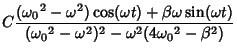
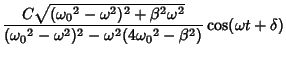
Using computer algebra to perform the algebra, the particular solution is
where
|
(84) |
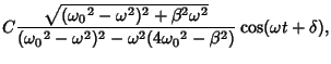
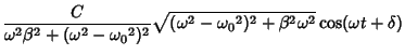
If the forcing function is sinusoidal instead of cosinusoidal, then
 |
(85) |
so
 |
(86) |
© 1996-9 Eric W. Weisstein
1999-05-26
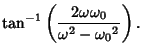
![$\displaystyle Ae^{-{\omega_0}t}\left[{-\int te^{{\omega_0}t}\cos(\omega t)\,dt+t\int e^{{\omega_0}t}\cos(\omega t)\,dt}\right]$](s1_1202.gif)
![$\displaystyle {A\over(\omega^2+{\omega_0}^2)^2}[({\omega_0}^2-\omega^2)\cos(\omega t)+2\omega{\omega_0}\sin(\omega t)].$](s1_1206.gif)

![$\displaystyle C {(\alpha^2+\gamma^2-\omega^2)\cos (\omega t)+2\alpha \omega\sin (\omega t)
\over [\alpha^2+(\gamma-\omega)^2][\alpha^2+(\gamma+\omega)^2]}$](s1_1300.gif)