|
|
|
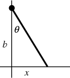
The Cauchy distribution, also called the Lorentzian Distribution, describes resonance behavior. It also describes the
distribution of horizontal distances at which a Line Segment tilted at a random Angle cuts the
x-Axis. Let ![]() represent the Angle that a line, with fixed point of rotation, makes
with the vertical axis, as shown above. Then
represent the Angle that a line, with fixed point of rotation, makes
with the vertical axis, as shown above. Then
| (1) | |||
| (2) | |||
 |
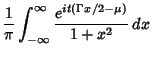
(3) |
| (4) |
 |
(5) |
 |
![$\displaystyle {1\over \pi}\left[{\tan^{-1}\left({b\over x}\right)}\right]_{-\infty}^\infty$](c1_608.gif) |
||
| (6) |
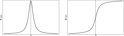
The general Cauchy distribution and its cumulative distribution can be written as
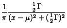 |
(7) | ||
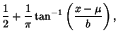 |
(8) |
 |
|||
 |
|||
| (9) |
| (10) | |||
 |
(11) | ||
| (12) |
| (13) | |||
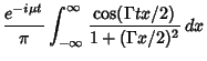
|
(14) | ||
| (15) |
If ![]() and
and ![]() are variates with a Normal Distribution, then
are variates with a Normal Distribution, then ![]() has a Cauchy distribution with
Mean
has a Cauchy distribution with
Mean ![]() and full width
and full width
| (16) |
See also Gaussian Distribution, Normal Distribution
References
Spiegel, M. R. Theory and Problems of Probability and Statistics. New York: McGraw-Hill, pp. 114-115, 1992.
|
|
|
© 1996-9 Eric W. Weisstein